Assessing Drift and Dispersion in Models of the St. Lawrence Estuary

– By Donovan Allum –

1. Introduction

The largest estuary in the world is the St. Lawrence Estuary and connects the – aptly named – St. Lawrence River to the Gulf of St. Lawrence and then the Atlantic Ocean. The river begins at Lake Ontario, passing important landmarks such as Kingston, Montreal, Trois-Rivières and Quebec City before emptying into the Gulf of St. Lawrence near the Gaspé Peninsula.

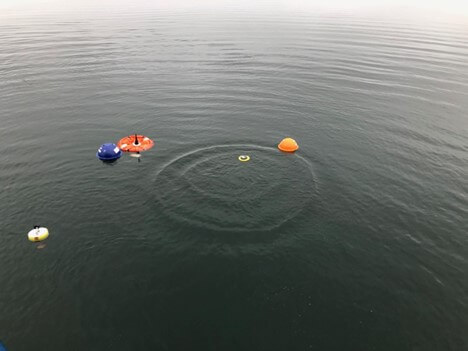
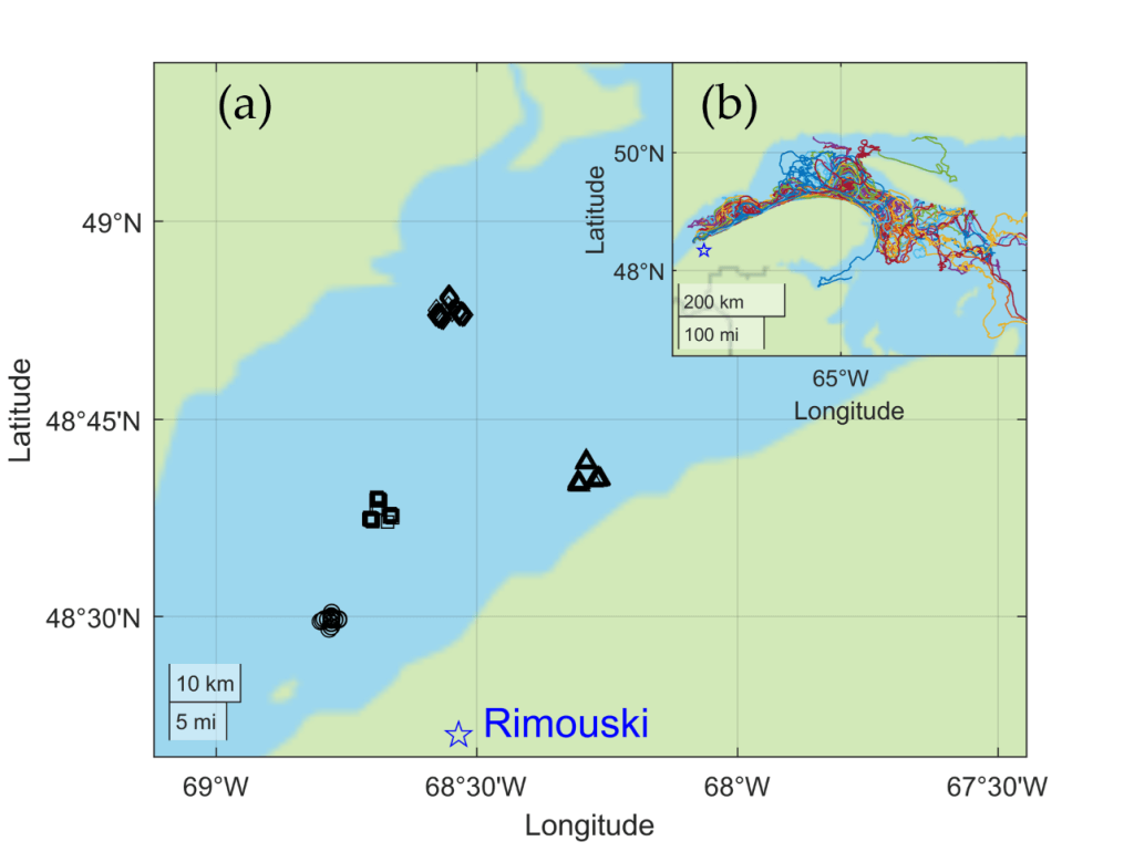
In 2020, 227 surface drifters (no deeper than 5 m) were released in the St. Lawrence Estuary, north of Rimouski, Quebec (Figure 2(a)) and continued downstream into the gulf of St. Lawrence, past Anticosti Island (Figure 2(b)). Most of the drifters were supplied by The Marine Environmental Observation, Prediction and Response Network (MEOPAR) and Réseau Québec Maritime (RQM). Additional drifters were provided by the Department of Fisheries and Oceans (DFO). The main goal of this experiment was to produce data to enable researchers to study drift and dispersion in the estuary for particles suspended at or near the surface with applications to search and rescue and environmental disturbances (like oil spills). There are approximately 2000 search and rescue incidents per year in the Maritime Rescue Sub-Centre (which includes the St. Lawrence Estuary). CBC also reports 334 oil spoils between 2002 and 2012 in the St. Lawrence River. As such, understanding drift and dispersion is of practical importance to the region.

The drifters tracked location versus time data, producing a large data set of particle trajectories freely floating down the estuary. Figure 2(b) shows the observed drifter paths of all 227 drifter trajectories that we used in our research. It would be ideal to release the drifters at or near the same time, but a project of this size on the estuary made this goal unfeasible. As a result, the bulk of the drifters were released gradually over 20 days, with several released even up to 50 days after the initial drop. This naturally complicates the project because we will be comparing drifters with different release positions and times.

My personal main area of research is the study of high-resolution simulations of hydrodynamics in cold water (i.e., water near the density maximum). This research seeks to create simulations that resolve all the scales of motion, from the largest to those at which dissipation takes place. Any study of a geographic region like the Gulf of St-Lawrence, cannot hope to resolve all scales of motion. Processes that occur below or near the grid scale are known as subgrid scale processes and they require parameterization to approximate their effect of these processes at the larger, resolved scales.

Due to the necessarily coarse resolution of these models, along with the probably imperfect parameterizations, modellers are always looking for methods to verify the accuracy of their models. Thanks to funding from MEOPAR and RQM, I was able to work on a project on field scales, more or less tangentially to my main area of research. The main goal of this project is to evaluate a particular measure of particle dispersion and assess the ability for models currently in use by the Government of Canada to predict drift and dispersion in the St. Lawrence Estuary.

Along with my PhD Supervisor Marek Stastna, we collaborated on this project with four employees of the Federal Government of Canada. Nancy Soontiens and Simon St. Onge-Drouin from Fisheries and Oceans Canada, and Christopher Subich and Graig Sutherland from Environment and Climate Change Canada. Regular meetings and discussions, both philosophical and practical, were instrumental to the success of this research.

2. Methods Used

There are many approaches and quantities that researchers use to attempt to quantify dispersion on different length scales. The simplest starting point considers single particle statistics, but this has two key drawbacks: (1) it cannot deal with particles released at different times, and (2) it does a poor job to quantify the spread of many particles, like in an oil spill. For this reason, the bulk of our work concentrated on the evolution of particle pairs.

The most natural quantity for studying particle pairs is known as the relative dispersion. If x_i is the position of the i‘th particle at time t, then the relative dispersion is
D(t) = ⟨(x_i-x_j)²⟩(t)          (1)
where the angled brackets indicate an average over all particle pairs. In layman’s terms, we quantify dispersion by analyzing the average, squared (so that it remains positive) particle-pair separation distance as a function of time. This measure is imperfect as well because it is an average over time and hence does not consider whether two particle pairs may be experiencing very different features of the flow, such as an eddy near a headland, that may be systematically moving particles.

Nevertheless, a similar quantity allows for a mathematical algorithm that quantifies separation across scales by averaging times at fixed distances instead of distances at fixed times. The process begins by setting a smallest separation distance, and defining larger and larger distances, each time multiplying by a scaling factor r. The algorithm computes what are called exit times (labelled T_i), or the times it takes for the separation distance to increase from one value to the next larger value. This is done for each particle pair, for each pair of separation distances and the exit time is averaged over all relevant particle pairs.

Of course, not all particle pairs achieve the largest distances, but the large number particles in our study made this a robust calculation. Finally, the so-called Finite Scale Lyapunov Exponent (FSLE) is defined
λ_i = [ln ln (r)] / [⟨T_i⟩]         (3)

The FSLE, λ_i, is a unique measure of dispersion because it can take discrete modelled or physical particle trajectory data and produce effective exponential separation rates. Even further, this quantity is useful to researchers because if λ_i obeys a power law according to D^-α (where D is the separation in km and α>0 is a constant), it can be argued that the relative dispersion scales as 2t^-α, where the parameter can depend on the separation scale. If i can be divided into regimes where α must take on different values, then it is often used to define dispersion regimes, where different phenomenon dominate separation on different scales.

The results from two numerical models were considered for this project. The first is the Coastal Ice-Ocean Prediction System (CIOPS-E). This model is a 1/36-degree model (2.5 km is a representative value) which extends from the St. Lawrence Estuary to the North Atlantic Ocean. The second model is the Gulf of St. Lawrence Ocean model (GSL). This model has a resolution of 500 m. Both models are coupled with an atmosphere model which interacts with ocean model to determine the modelled ocean currents.

Model particle trajectories starting in the same positions as in the TReX project (Figure 2(a)) were produced by collaborators Soontiens and Sutherland. These were subsequently used to compute FSLE.

3. What We Found

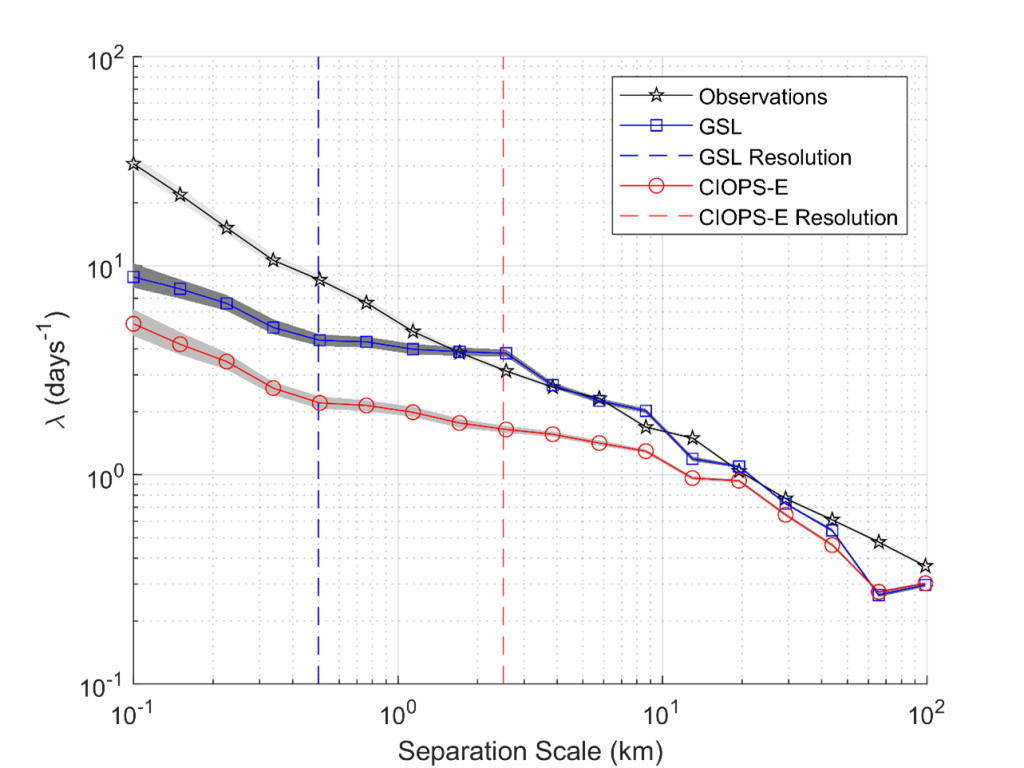
For each model and the observed drifter paths, we calculated the FSLE over length scales of 0.1 km to 100 km with r=1.5 (Figure 3). It is presented in this Figure on a log-log scale because if the FSLE behaves as a power-law like D^-α, then the FSLE will be a straight line on a log-log scale. Different slopes define different dispersion regimes. There are three main observations to make about Figure 3: (1) the FSLE of the observations is approximately constantly in slope, (2) both models produce smaller FSLE in magnitude and shallower slopes than the observed FSLE at small length scales, and (3) both models produce similar slopes and magnitude compared to the observations at large length scales.

The consistent slope of the observations suggests that the separation rate is consistent on all scales considered and the entire estuary – over the scales considered – is in a single dispersion regime. In other words, the average drifter pair at a length scale of 0.1 km is separating in a similar manner to the average drifter pair separated by 50 km. This is a surprising statement for two reasons. Firstly, many features of the flow are wildly different on 0.1 km and 100 km separation scales. Secondly, unlike in the open ocean – where the FSLE is most often used – the estuary is bounded by the shore at ~40-50 km. We expected changes to the FSLE to occur at length scales corresponding to features in the estuary currents and near the estuary width.

Both numerical models exhibit smaller FSLE – and hence, longer exit times – at small length scales compared to the observed FSLE. The slopes are consistent between models and shallower than their observed counterparts. The GSL model produces larger FSLE in magnitude than the CIOPS-E model. This is a really interesting difference between the two models which is likely caused by the difference in resolution. Determining the source of this difference could be an interesting avenue for future research.

The standard interpretation of the shallower slope in both models is that dispersion is different at small scales in the models than it is for physical drifter pairs. This is unsurprising that there is a difference in some kind, in part because some of these length scales are below the grid resolution of the models. It is, however, surprising that the models systematically produce smaller FSLE, and hence longer separation times. Due to some complicated details about how the modelled trajectories were obtained, it is possible for modelled drifters to occupy space between grid points allowing for separations below the grid spacing (indicated by the vertical dashed lines in Figure 3 for each model).

Information about how the models will handle dispersion at length scales below the grid resolution is important because real phenomenon like oil spills or search and rescue situations happen on scales below 1 km. According to the FSLE in Figure 3, the models significantly underestimate the separation rates at small scales. This would be especially problematic in a search and rescue operation where it is imperative to define a search region based on a theoretical maximum distance that a floating object could have drifted following an accident or crash.

At large length scales, the FSLE of the models behave very similarly, matching the observed FSLE in slope and magnitude quite well. Except for the dip near 70 km. It is not surprising that the dispersion would behave similarly at larger length scales. It is generally agreed that at large enough length scales, ocean models should accurately reproduce reality. This is known as an “effective resolution”, distinct from the true resolution which is determined by the grid spacing. An effective resolution depends on the phenomenon being measured.

Where the comparison between models is most interesting is between the smallest and largest length scales, and how the two models transition from disagreement to near agreement with the observations at large scales. The GSL model transitions to match the observations – in slope and magnitude – at a smaller separation scale than the CIOPS-E model. It may be possible to use the FSLE to estimate an effective resolution of each model for dispersion. From Figure 3, a reasonable estimate of the effective resolution would be 2-3 km for the GSL model and 10-20 km for the CIOPS-E model. By this measure, the GSL model requires 2-3 km separations before dispersion is accurately captured. Similarly, for the CIOPS-E model.

Figure 3 also includes 99% confidence intervals for each data set which shows the robustness of this measure applied to this data set.

4. Conclusions

We were able to take the observed particle trajectories and compress them into a single line plot using the FSLE algorithm that converted separation distances between particle pairs into effective exponential separation rates. Through the use of a 99% bootstrapped confidence interval, we demonstrated that this calculation is robust despite the fact that drifters were released over a long period (as long as 50 days) and non-uniformly about the estuary.

We then calculated the FSLE for the GSL and CIOPS-E models with drifters released from the same locations as the observed drifters. We found that at small length scales, the modelled FSLE differed from the observed FSLE with a small magnitude and shallower slope. At larger length scales both models more accurately with the observations.

What does this mean for search and rescue or oil spill response teams who use these models? Real drifters are separating from each other more rapidly than modelled equivalent. It is unsurprising that there would be differences at length scales below the modelled resolution, but this result specifically argues that the models are predicting dispersion that is significantly slower than reality at small length scales which are most relevant immediately after a spill or crash. For a more complete and technical analysis of these results, our team is currently working on a paper which will be submitted this year.

Donovan Allum is a 3rd year PhD student at the University of Waterloo in Applied Math. His main area of research is high resolution fluid mechanical simulations below the temperature of maximum density. He started work on this project in May 2021 and hopes to publish this research soon.