Is global warming causing Atlantification of the Barents Sea, a collapse of the North Atlantic currents, or neither?

Written by CMOS Bulletin SCMO on October 22, 2023. Posted in Climate, Oceans, What's Current.

– By Knut L. Seip and Hui Wang –

This study is about the Barents Sea and two North Atlantic currents, the Atlantic meridional overturning circulation (AMOC) and the Atlantic multidecadal oscillation (AMO) and what happens when the North Atlantic currents reach the Barents Sea.

Figure 1. The warm surface water that comes from the Caribbean turns away from Canada and reaches Europe before it meets the Barents Sea North of Norway. The Barents Sea is cold and is feed by ice breaking off from the North Pole ice cover.

Why are the AMO and the AMOC important?

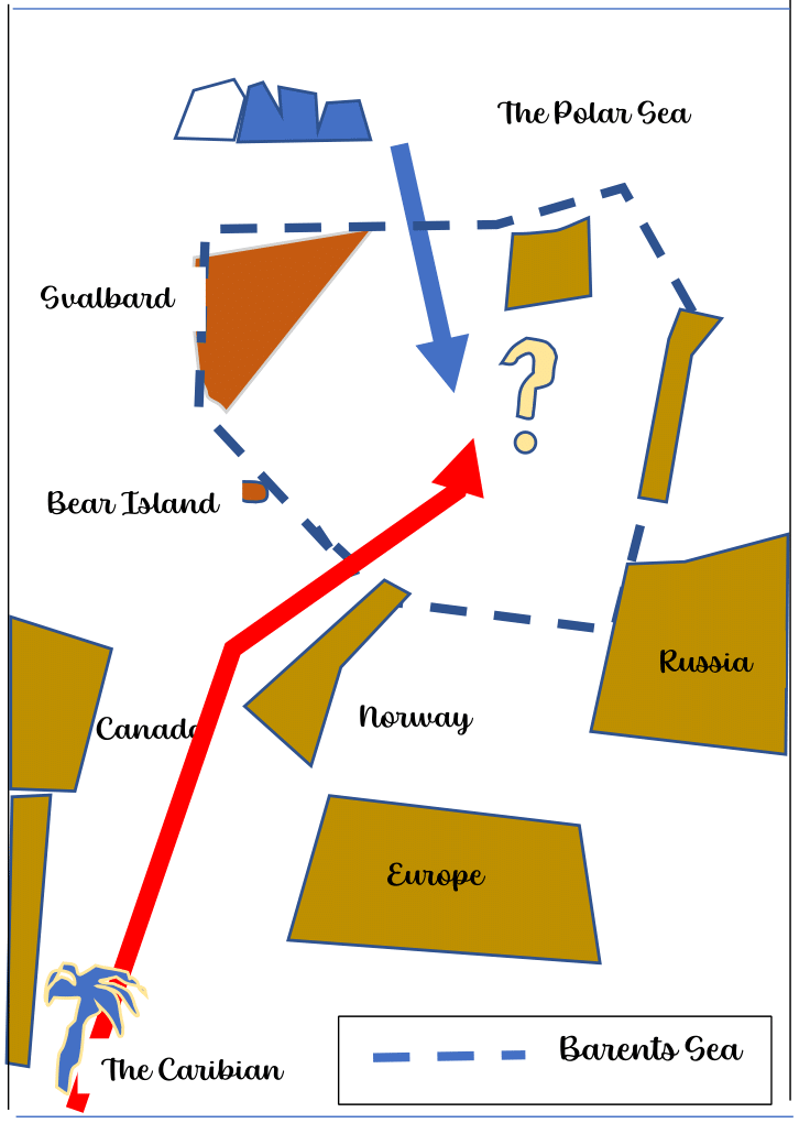
The AMO and the AMOC are two currents that are shown to strongly impact the climate on the Northern Hemisphere. The trajectory for the AMOC is sketched in Figure 1. Warm currents, like the Gulf Stream, which are part of the AMOC, are coming from the Caribbean and meet cold water in the Barents Sea. Three major effects from AMO and AMOC on the Barents Sea are suggested because of global warming. First, the Barents Sea will be Atlantificatied (Barton et al. 2018) and the ecosystem of the Barents Sea will be similar to that of the North Atlantic (Ingvaldsen et al. 2021). Second, the cold and ice fed water in the Barents Sea moves into the North Atlantic and changes the Atlantic currents dramatically. In an extreme scenario, the AMOC will collapse (Ditlevsen and Ditlevsen 2023) and a sudden and severe decrease in temperature across northern Europe and the United States can occur. The third scenario is that there is no effect from the Barents Sea on the AMOC and AMO (Li et al. 2021) or vice versa.

How to get closer to the answer

Since ocean currents show variability (most probably with pseudo cycles), we can assume that a peak in the causal variable would occur before a peak in the effect variable. Therefore, if AMOC peaks before cycles peak in the Barents Sea, we interpret this as meaning that the temperatures in the Atlantic waters impact the temperature in the waters of the Barents Sea. If AMOC peaks after the current peaks in the Barents Sea, then it is the Barents Sea that affects the North Atlantic waters and the AMOC.

The real story is a little bit more complicated. The AMOC is measured in cubic meters per second (Sv), the AMO in ^oC, and salinity also plays a role. However, here we focus on the temperature part and on AMOC.

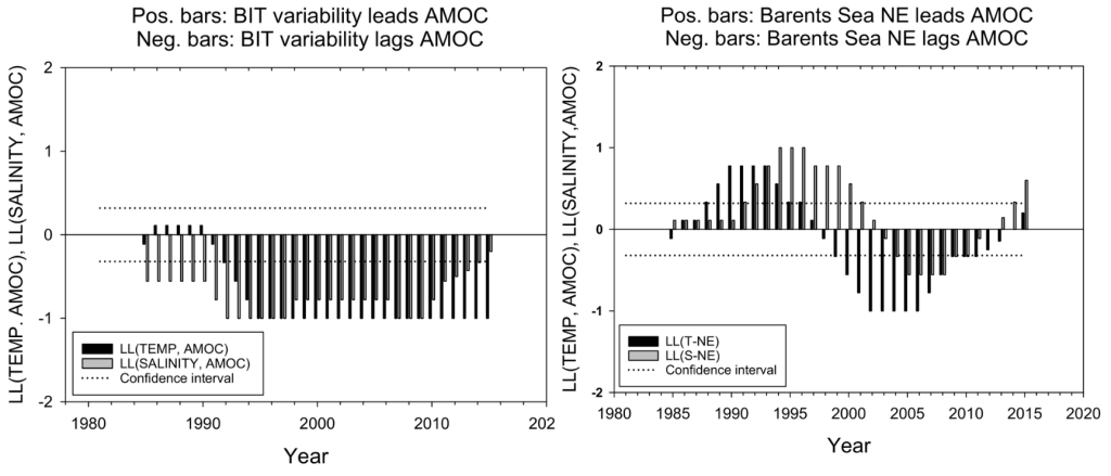
To use the information on lead and lag (LL) relations between ocean currents, you need a method that quantifies LL relations over very short time spans. The trick to do that is explained in the method section below. To test if the result is significant, we do as one always does. We compare the persistence of an LL relation to that of two stochastic series. The more persistent a leading relation is, the more confident we are in its causal effect. And it is even better if the cycle periods change in duration (the series are non-stationary), and the two series still show persistent LL relations. To show the resulting LL relations between two time series, we use a graph with bars that are either positive (the first series leads the second) or negative (the second series leads the first) in Figure 2.

We got two results

We examine two inlets for the AMOC to the Barents Sea. The peaks in the AMOC series came before the peaks in the currents that was observed in the Bear Island trough (BIT, one of the inlets) from the year 1991 to 2014, that is 23 years, Figure 2a. However, in the inlet at the Barents Sea northeast (BSNE), there is first a short period of 6 years where the Barents Sea currents lead the AMOC, but then a second short period of 8 years where the AMOC leads the Barents Sea currents, Figure 2b.

Figure 2. The AMOC and the currents in the Barents Sea outlets meet each other. a) In the Bear Island trough (BIT) at about 400-m depth. The negative bars mean that for the period 19912014, the AMOC was significantly leading currents in the Bear Island trough and salinity was doing the same. b) In the Barents Sea northeast the lead-lag patterns are more complex, and salinity and temperature do not follow each other as closely as at the BIT (Yashayaev (2015) observed that temperatures lead salinity as in the first half of the time in Figure b.) The dashed lines denote approximate confidence limits.

Time series for heat and salinity transport between the North Atlantic waters and the Barents Sea are based on observations. Our results and interpretation of the data suggest that heat and salt are transported both ways, and with different timing at the two regions where the AMOC meets the Barents Sea.

If we assume that the water flows through the two inlets are similar in size, then it is the inflow at the BIT, that is, the water carried with the AMOC and the AMO that dominates the waters in the Barents Sea during the period 1971 to 2014. The inlet through the BIT may have a larger cross section than the inlet at the BSNE (Barton et al. 2018).

We also obtained a second result. We found that temperature variations in the surface water of the Barents Sea always lead the temperature variations in the intermediate water, suggesting that heat variations in the atmosphere are transported to the Barents Sea waters (graphs not shown).

Our conclusion is that temperatures in the Barents Sea are influenced by temperature variations in the atmosphere and by temperature variations in the North Atlantic waters (the AMOC and the AMO) until about 2000. In addition, temperature variations within the Barents Sea are caused by ice melting and accompanying changes in albedo. After about 2018 global warming may play an increasingly important role in the Barents Sea-North Atlantic Ocean system.

There are four caveats in our results. i) The assumption that the flow through the BIT is larger or of about equal size to the flow through the BSNE may not be correct, and there are more gateways to the Barents Sea than those two studied here. ii) The study period was only 48 years, and ocean currents may change directions after that time (Seip et al. 2023). iii) Global warming may alter ocean flow patterns in the Barents Sea and in the North Atlantic. In particular, the return flow of cold-water at large depths may change characteristics. iv) Last, the atmosphere-ocean exchange of heat may change with global warming and global cooling (Li et al. 2023).

The method trick

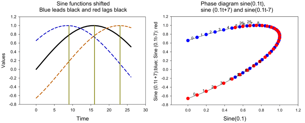
The trick to distinguish lead-lag patterns is to depict the potential causal and effect series in a phase plot. In such a plot, we can determine the lead-lag pattern based on three paired consecutive observations (and not only for the peaks or troughs). Figure 3 shows that if one time series peaks before another (blue and black in Figure 3, black on the x-axis), then the trajectories rotate clockwise. If one time series peaks after another (black and red, black on the x-axis), then the trajectories rotate counterclockwise.

Although it may be easy to see the relation between series in a phase diagram, the equation that calculates rotational directions in the phase diagram could be difficult to write out. For readers that are interested we would be glad to provide a one-page spread sheet (Excel book) with the appropriate calculations. Then, to use the method, just paste the time series into two columns in the spread sheet.

Figure 3. The trick: How to know which series is leading which. a) Three series, the blue series leads the black series because it peaks before the black series, the red series trails the black series because it peaks after the black series. b) Phase plot with sine (0.1t) on the x-axis and sine(0.1t+7): blue and sine (0.1t-7): red on the y-axis.

Knut L. Seip is professor emeritus at Oslo Metropolitan University. He has recently been working on aquatic and economic problems using a high-resolution lead-lag (cause before effect) methodology to disentangle causal variable in observed time series.

Hui Wang is a meteorologist from the Climate Prediction Center of the U.S. National Oceanic and Atmospheric Administration. His research interests are climate variability, climate modelling and prediction.

References

Barton, B. I., Y. D. Lenn and C. Lique (2018). “Observed Atlantification of the Barents Sea Causes the Polar Front to Limit the Expansion of Winter Sea Ice.” Journal of Physical Oceanography 48(8): 1849-1866.

Ditlevsen, P. and S. Ditlevsen (2023). “Warning of a forthcoming collapse of the Atlantic meridional overturning circulation.” Nature Communications 14(1).

Ingvaldsen, R. B., K. M. Assmann, R. Primicerio, M. Fossheim, I. V. Polyakov and A. V. Dolgov (2021). “Physical manifestations and ecological implications of Arctic Atlantification.” Nature Reviews Earth & Environment 2(12): 874-889.

Li, F., M. S. Lozier, S. Bacon, A. S. Bower, S. A. Cunningham, M. F. de Jong, B. DeYoung, N. Fraser, N. Fried, G. Han, N. P. Holliday, J. Holte, L. Houpert, M. E. Inall, W. E. Johns, S. Jones, C. Johnson, J. Karstensen, I. A. Le Bras, P. Lherminier, X. Lin, H. Mercier, M. Oltmanns, A. Pacini, T. Petit, R. S. Pickart, D. Rayner, F. Straneo, V. Thierry, M. Visbeck, I. Yashayaev and C. Zhou (2021). “Subpolar North Atlantic western boundary density anomalies and the Meridional Overturning Circulation.” Nature Communications 12(1).

Li, H., J. Richter, H, A. Hu, G. A. Meehl and D. MacMartin (2023). “Responses in the subpolar North Atlantic in two climate model sensitivity experiments with increased stratospheric aerosols.” Journal of Climate: 1-31.

Seip, K. L., Ø. Grøn and H. Wang (2023). “Global lead‑lag changes between climate variability series coincide with major phase shifts in the Pacific decadal oscillation.” Theoretical and Applied climatology.

0 Shares

Atlantic meridional overturning circulation, Atlantic multidecadal oscillation, Barents Sea, Hui Wang, Knut Seip, North Atlantic, Oceans