Micrometeorological Variables and Atmospheric Dispersion Modeling in Two Climate Regions of Quebec

Written by CMOS Bulletin SCMO on July 27, 2020. Posted in Air Quality, Atmosphere, Climate, Weather, What's Current.

– By Richard Leduc, Ph.D., AirMet Science Inc., and Jean-François Brière, Ministère de l’Environnement et de la Lutte contre les changements climatiques

The US-EPA (2019a) AERMOD dispersion model is widely used to assess the concentration of contaminants in ambient air as a result of emissions from a source. To this end, AERMOD requires micrometeorological variables characterizing turbulence (u*, w*, L, zic, zim); they are calculated by the AERMET module and obtained using local surface and upper air data (wind, temperature and cloud opacity), the calculation details of which are in EPA (2019b). Climatic differences will thus affect these variables and influence atmospheric dispersion. Two stations (Maniwaki and Sept-Îles) located in two different climatic regions of Quebec and separated by a distance of about 800 km were selected in order to compare their micrometeorological variables and the results of the dispersion modeling from a point source emission for the 2008-2012 period. Results from this comparison are briefly presented here; more detailed results are available by contacting an author.

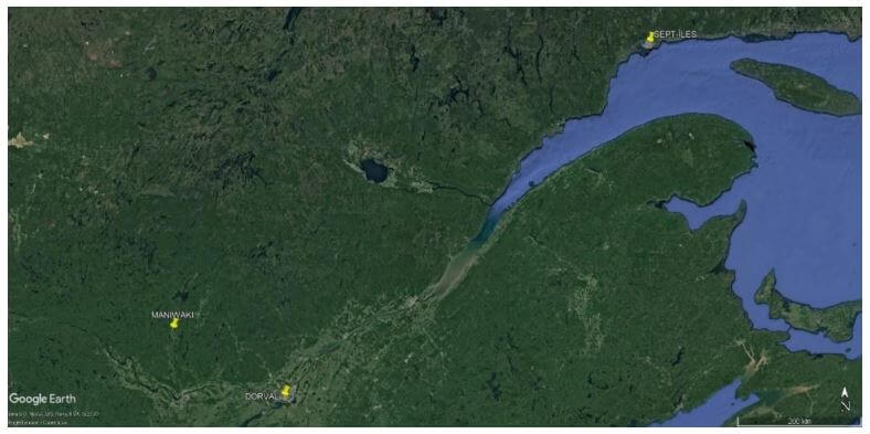
Figure 1. Dorval, Maniwaki, and Sept-Îles locations

Sept-Îles is colder than Maniwaki with an annual average of 2.8°C compared to 5.5°C. A clear sky is less frequent in Sept-Îles than in Maniwaki (17.04% vs 20.15%) and the opposite is true for a covered sky with an opacity of 10 (33.53% vs 30.54%). Excluding calm winds for which calculations are not made, the average wind speed in Sept-Îles is higher than at Maniwaki (4.49 m/s vs 2.24 m/s) and it is the same for the friction velocity (u*; 0.29 m/s vs 0.22 m/s); results are also compared using Q-Q plots (Figure 2 with 1st, 2nd, 5th, 10th, 15th,…, 95th, 98th, 99.5th and 100th percentiles). Percentiles for u* are higher in Sept-Îles.

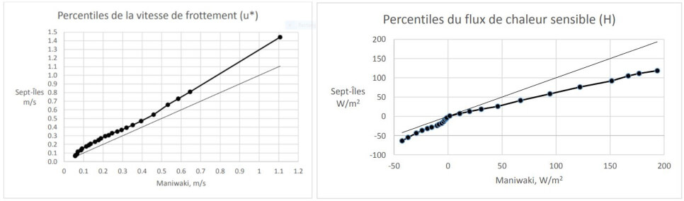
(Left) Figure 2. Percentile of shear velocity u* (m/s) -Sept-Îles – Maniwaki
(Right) Figure 3. Sensible heat flux percentiles (W/m²) – Sept-Îles – Maniwaki

The higher latitude, the greater cloudiness and the lower temperature of Sept-Îles produce differences in the sensible heat flux (H) so that Maniwaki’s average is much higher (16.47 W/m² vs 1.11 W/m²); it is seen (Figure 3) that percentiles are not much different for H<0 W/m² (60th percentiles) but the difference gets higher after.

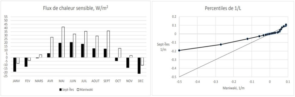
(Left) Figure 4. Monthly sensible heat flux (W/m²)
(Right) Figure 5. Percentiles of 1/L (m-¹) – Sept-Îles and Maniwaki

The distribution of 1/L (Figure 5) show values in Sept-Îles that are much less negative than in Maniwaki up to the 45th percentile and after positive values higher in Maniwaki up to the 90th percentile and finally those of Sept-Îles are a little higher. To distinguish the between the stability conditions, a range of -0.015 m-¹ to 0.015 m-¹ was chosen for a neutral class; the frequency of neutral cases is 53% in Sept-Îles and 28% in Maniwaki, while convective cases (<-0.015 m-¹ ) are more frequent in Maniwaki (25% vs 16%) and also for the stable cases (> 0.015 m-¹; 46% vs 31%). These results are attributable to a windier and cloudier conditions in Sept-Îles.

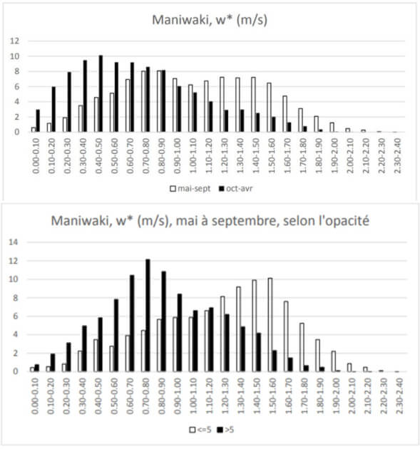
Figure 6. Percentiles of w* (m/s) Sept-Îles and Maniwaki

(Top) Figure 7. Histogram of w* in Maniwaki for two seasons
(Bottom) Figure 8. Histogram of w* in Maniwaki during the warm season (May to September) based on opacity

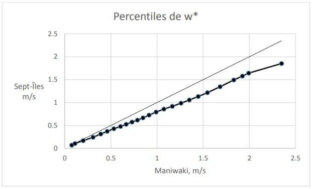
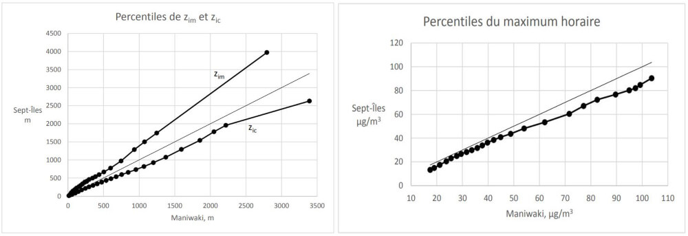
In Maniwaki, the mean convective velocity scale (w*) is higher than that of Sept-Îles (0.9 m/s vs 0.71 m/s) as shown also in Figure 6. The distribution of w* in two seasons (May to September and October to April) and also in the warm season according to cloud cover opacity are quite different (Figure 7, Figure 8); similar results are obtained for Sept-Îles. The average convective mixing height is greater in Maniwaki (647.3 m vs 519.6 m) and it is the contrary for the mechanical mixing height (273.5 m vs 403.3 m); these differences are also shown in Figure 9.

(Left) Figure 9. Percentiles of zim (m) and zic (m)
(Right) Figure 10. Percentiles of hourly maximum concentrations

The micrometeorological variables of Maniwaki and Sept-Îles are used to model (with AERMOD) the atmospheric dispersion of emissions from a point source (h_s=15 m, d_s=0.5 m, v_s=10 m/s, T_s=50°C, q_s=1 g/s) in order to examine how they influence the concentrations calculated at 4481 receptors over the same 5 years period.

In Maniwaki, the highest hourly concentration is 103.69 μg/m³ compared to 90.43 μg/m³ in Sept-Îles (+14.7%). The average hourly maxima for all receptors is 14% higher in Maniwaki (46.83 μg/m³ vs 41.06 μg/m³). The highest 99.5 hourly percentile is 62.92 μg/m³ in Maniwaki and 47.86 μg/m³ at Sept-Îles (+31.5%) and the percentiles of the hourly maximum are higher in Maniwaki (Figure 10).

With respect to daily maxima (Figure 11), Sept-Îles is at 30.73 μg/m³ compared to 43.09 μg/m³ in Maniwaki (+40.2%); it is the same for the mean and the median (+55.7%, +44.5%).

The maximum mean of the period is 3.45 μg/m3 in Sept-Îles and 4.29 μg/m3 in Maniwaki (+24.3%); over all receptors, Maniwaki has a mean 83% higher (0.97 μg/m³ vs 0.53 μg/m³) and the median is 31.1% higher (0.59 μg/m³ vs 0.45 μg/m³); Figure 12 also shows the greater difference between the two places.

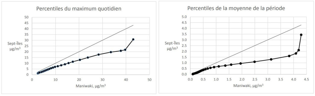
(Left) Figure 11. Percentiles of daily maximum concentrations
(Right) Figure 12. Percentiles of mean concentrations for the time frame

For all receptors, hourly maximum concentrations in Sept-Îles are mostly associated with neutral conditions (about 41%), while in Maniwaki it’s mostly stable conditions (about 47%), which may be the cause of its more elevated concentrations calculated there.

In conclusion, the impact of climatic differences between Dorval and Sept-Îles on micrometeorological variables has been quantified, which in turn produced different dispersion modeling calculation results. Different results could also be obtained for other source types, such as surface sources and other local conditions such as topography.

ACKNOWLEDGEMENTS

We express our sincere thanks to M. Philippe Barnéoud, Environment and Climate Change Canada, for his advice and comments and Lakes Environmental for the usage of AERMOD-View.

REFERENCES

EPA, 2019 a: AERMOD Model Formulation and Evaluation. EPA-454/R-19-014, August 2019, 177 p.
EPA, 2019 b: User’s Guide for the AERMOD Meteorological Preprocessor (AERMET). EPA454/B-19-028, August 2019, p.310
Panofsky, H.A., J.A. Dutton, 1984: Atmospheric Turbulence. Models and Methods for Engineering Applications. J. Wiley & Sons, p.397.

About the Authors

Richard Leduc

Richard Leduc began his career in 1972 in Downsview. In 1979, he joined Environment Quebec where he worked for 28 years in Air Quality (network monitoring modelling and applications). He is an Associate Professor (volunteer) at Laval University. For the last 13 years, he’s worked with AirMet Science Inc. He can be reached at rleduc@airmetscience.com.

Jean-Francois Briere

Jean-François Brière holds a Bachelor’s and Master’s in Physics from Laval University. He has been an employee with the Ministry of Environment and Climate Change since 2009. He worked for nine years as an Atmospheric Dispersion Modeler, and since 2017, he’s been the team lead on atmospheric dispersion modeling and atmospheric quality standards and criteria. He can be reached at Jean-Francois.Briere@environnement.gouv.qc.ca.

Did you enjoy this article? Subscribe here to get the latest from the CMOS Bulletin!

More Like This:

0 Shares

AERMOD dispersion model, emissions from a source, Jean-François Brière, micrometeorological variables, Richard Leduc